

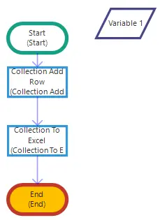


This activity creates a new worksheet within an existing Excel workbook. It is commonly used to generate structured output, reporting, or temporary working sheets during automation.
Usage Scenarios
Creating a new sheet to store automation results
Adding a dedicated sheet for processing without modifying the original template
Generating report, analysis, or staging sheets dynamically
Naming sheets by date, user, or process for tracking purposes
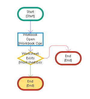
Automatically creating a sheet if it does not already exist (used with Worksheet Exists)
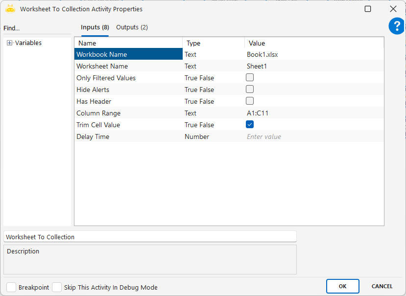
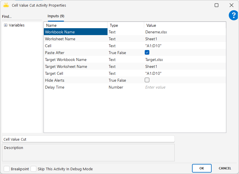
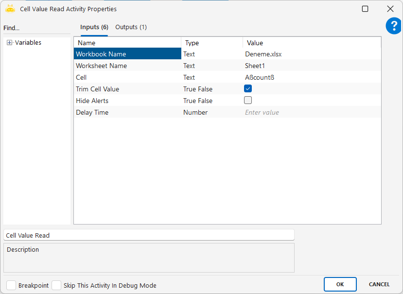
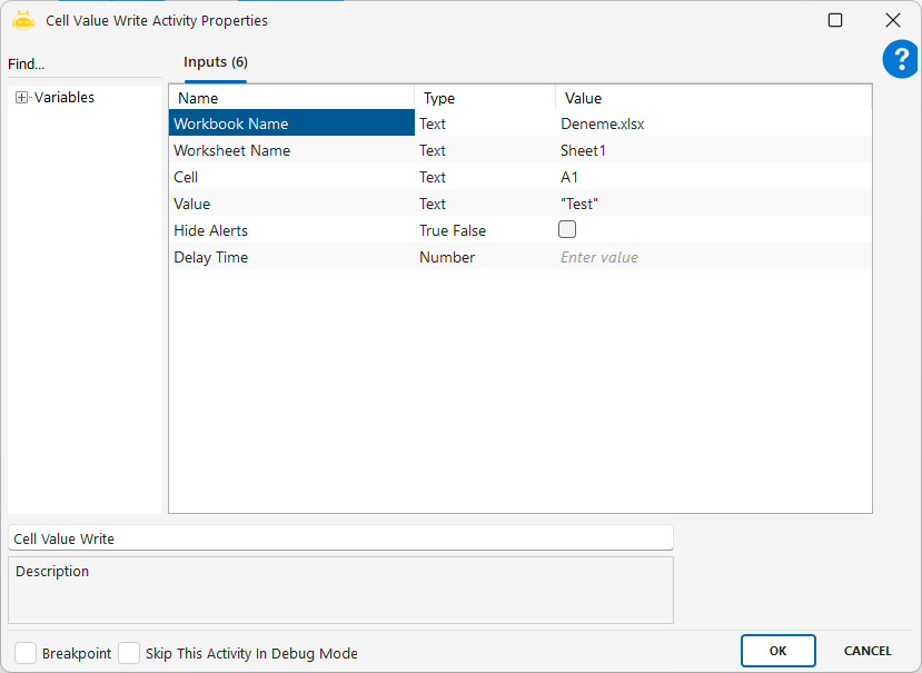
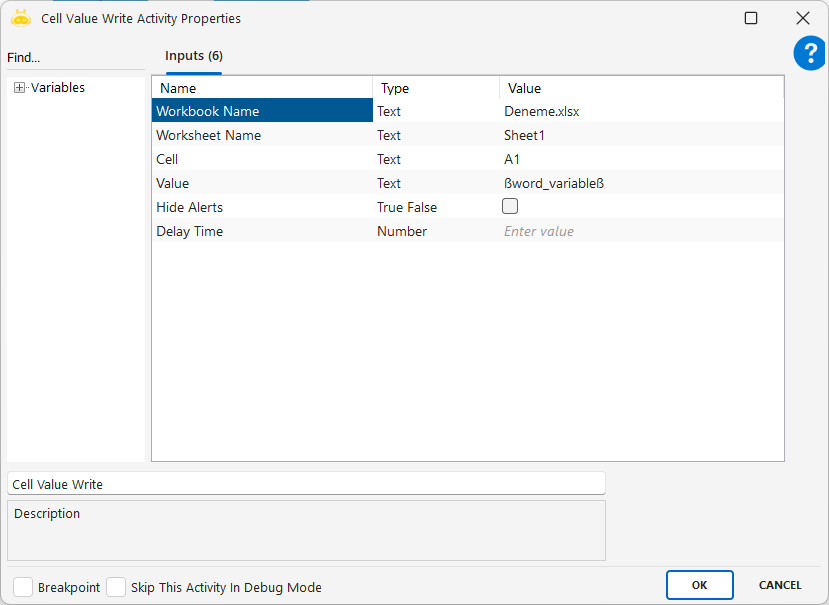
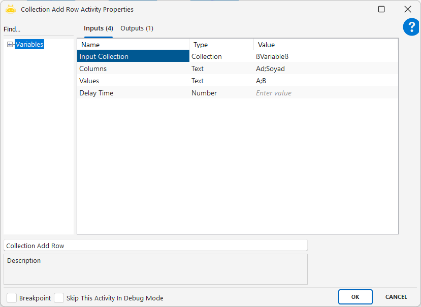
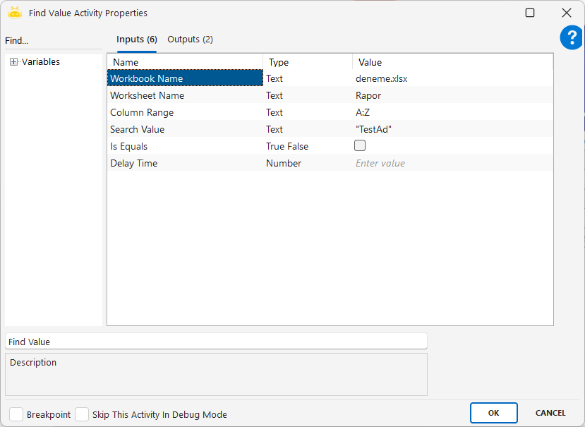
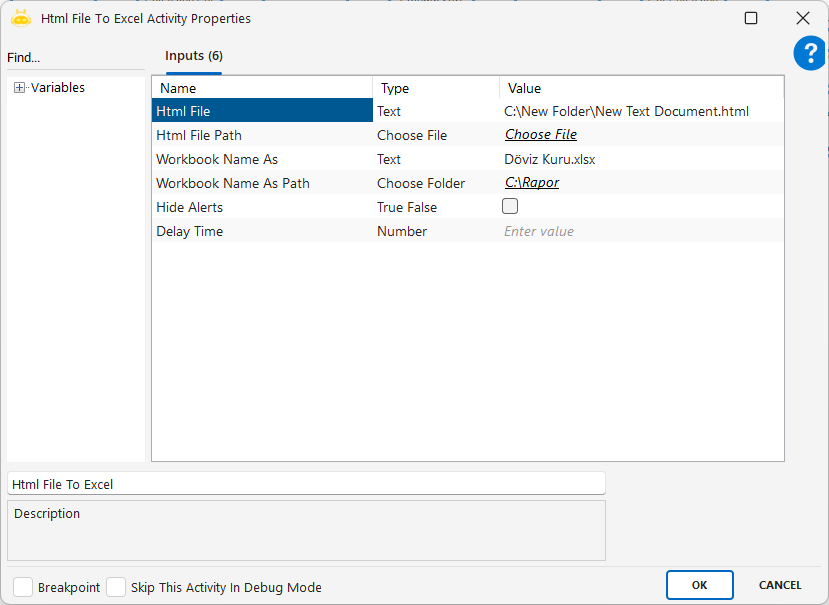
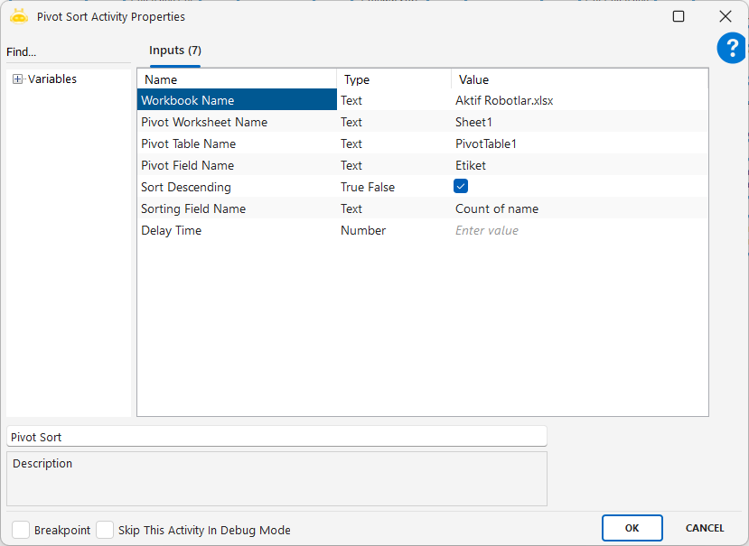
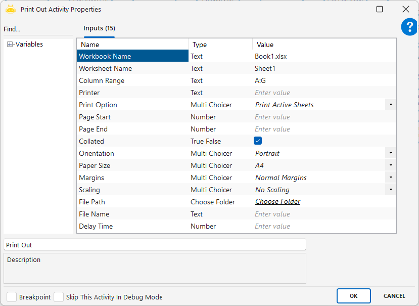
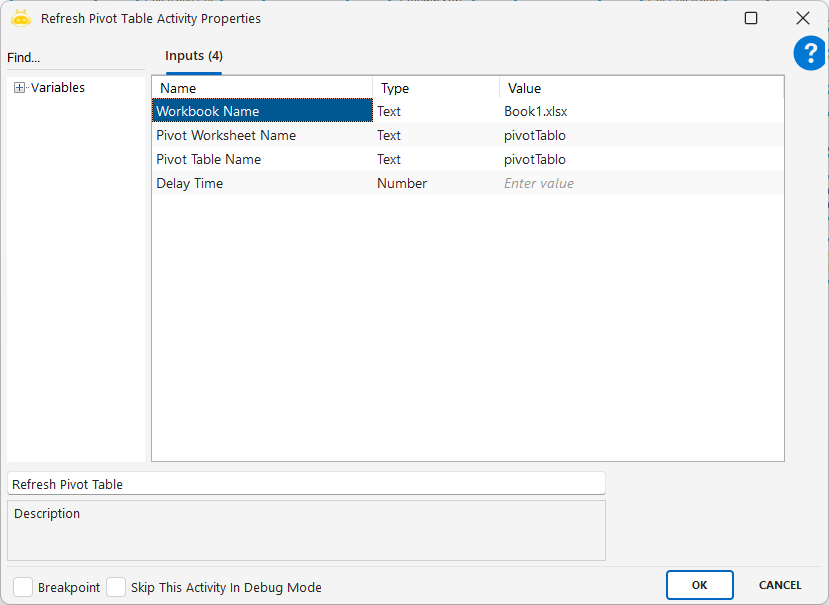
Parameters
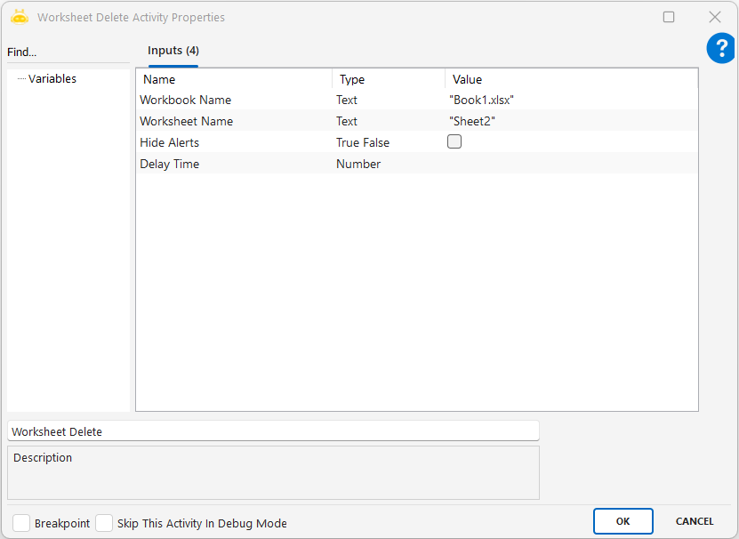
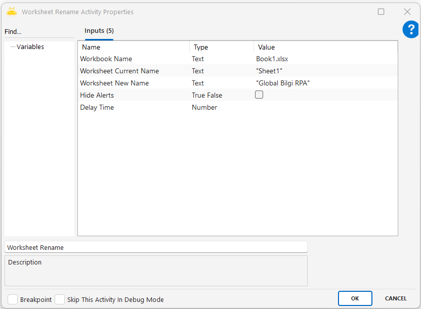
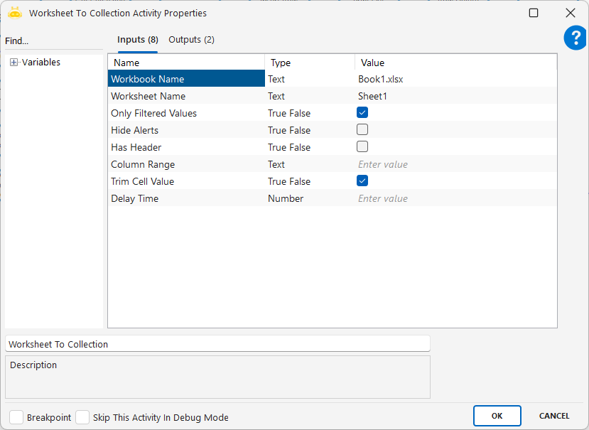
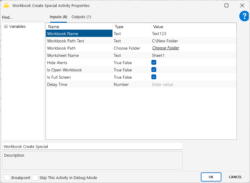
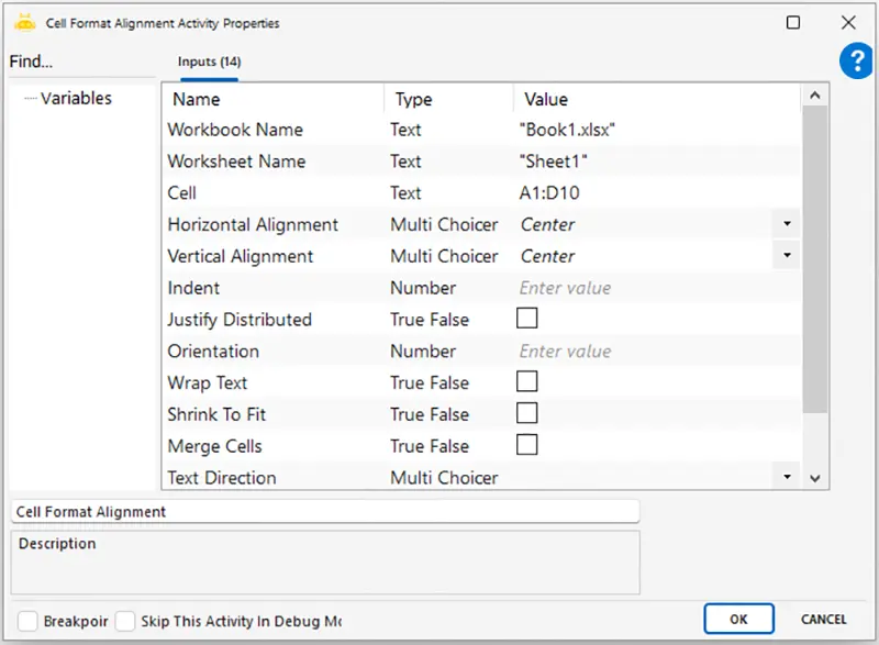
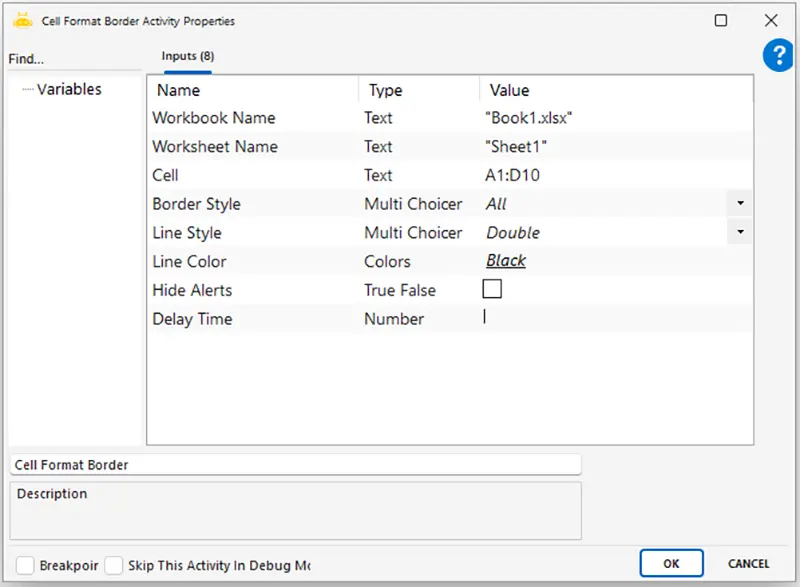
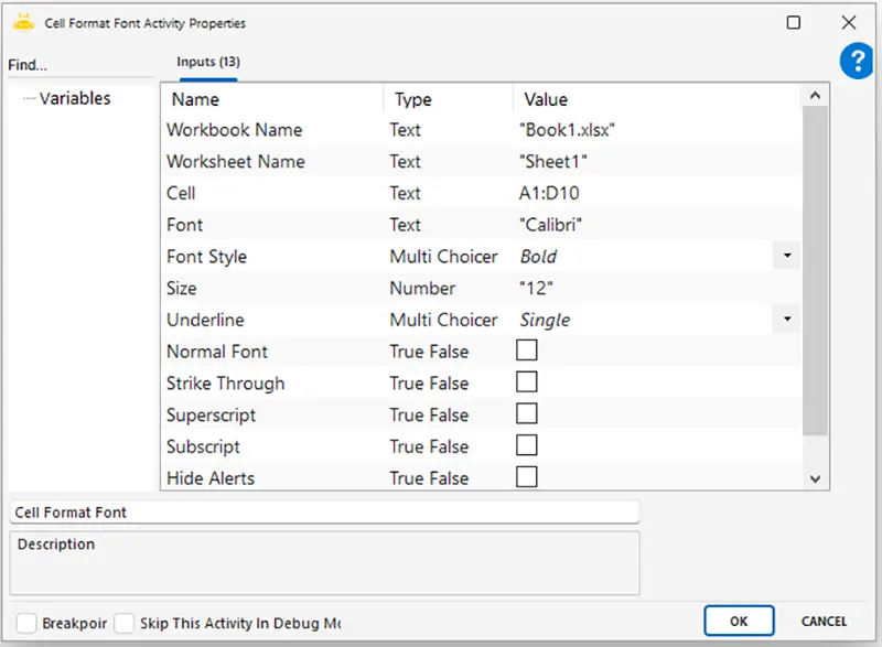
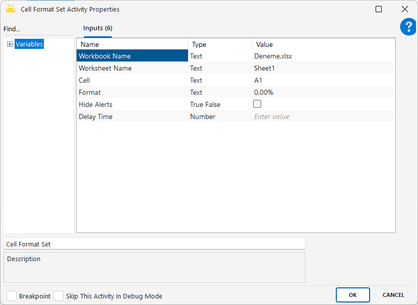
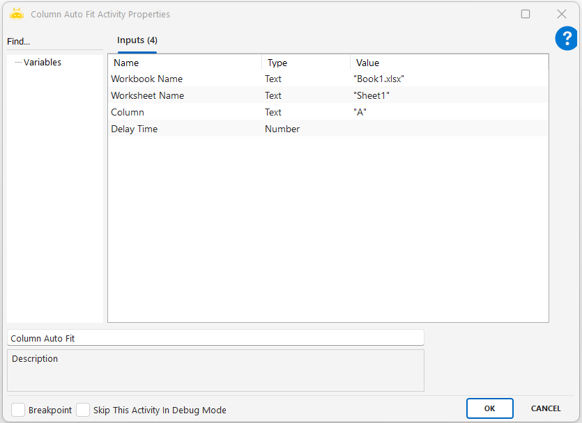
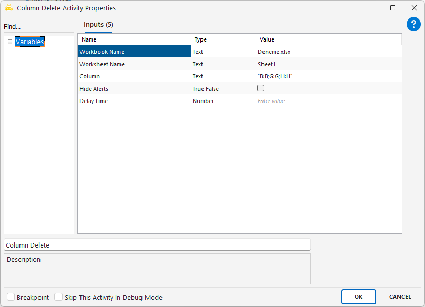
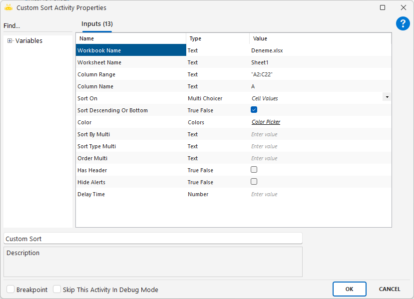
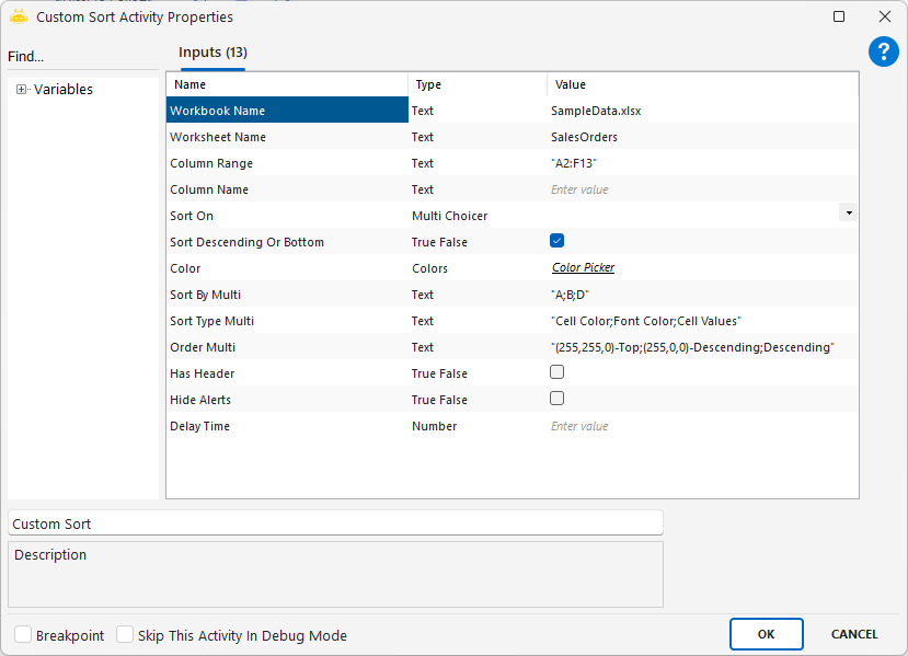
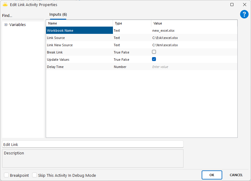
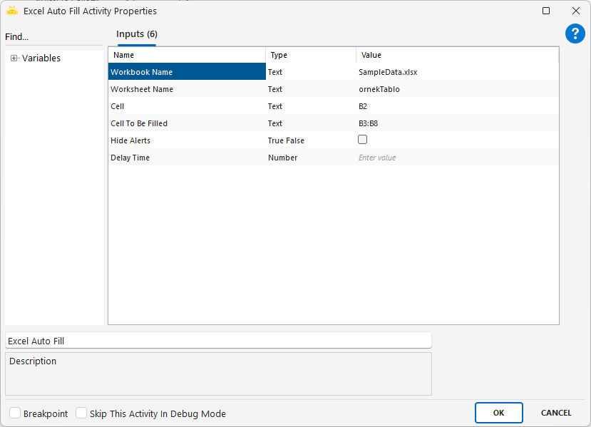
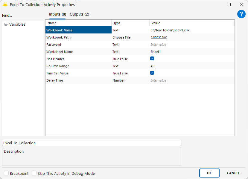
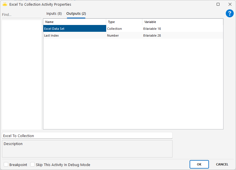
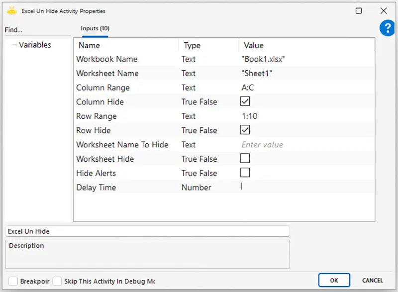
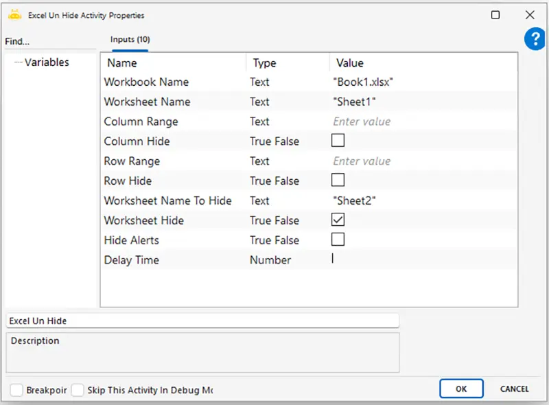
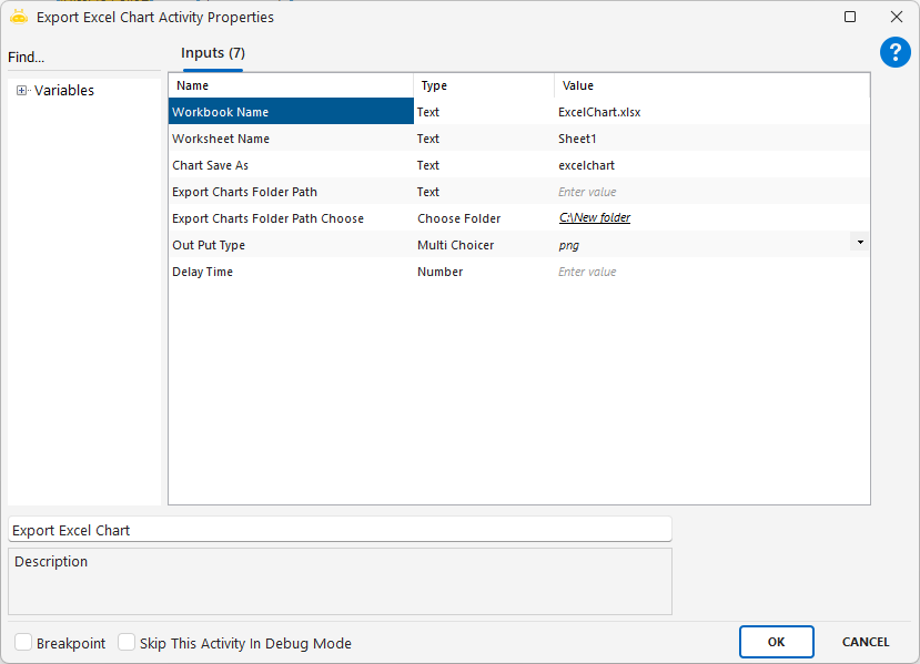
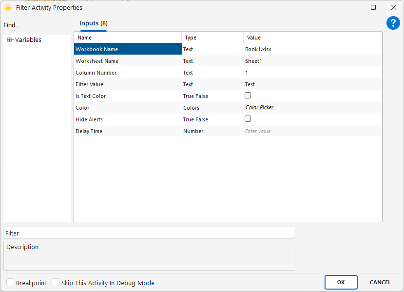
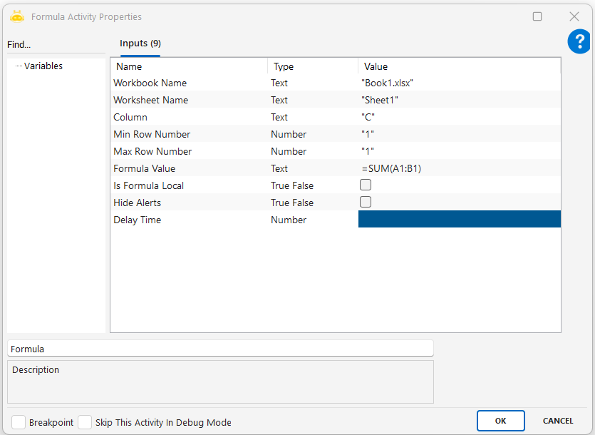
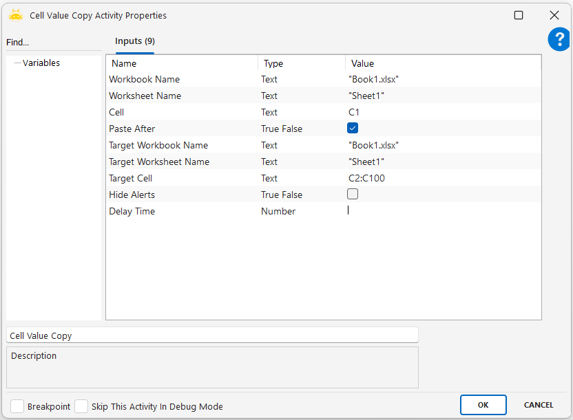
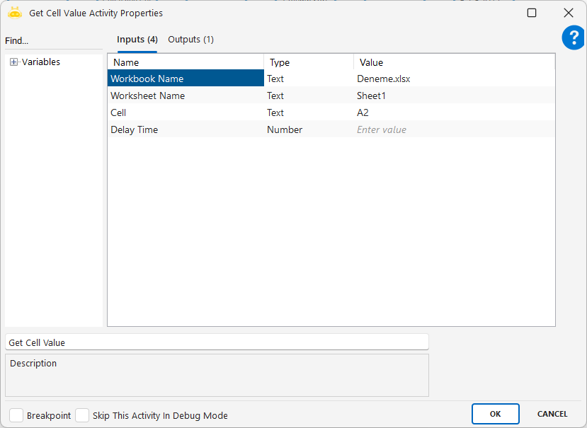
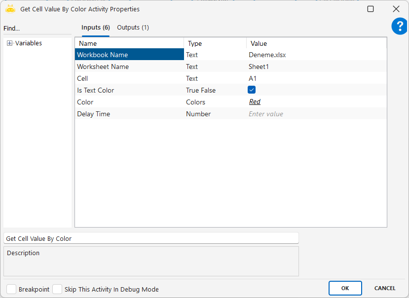
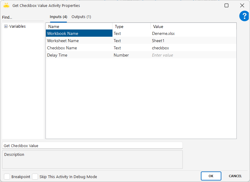
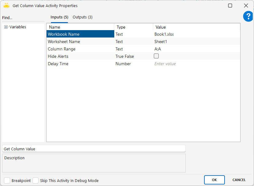
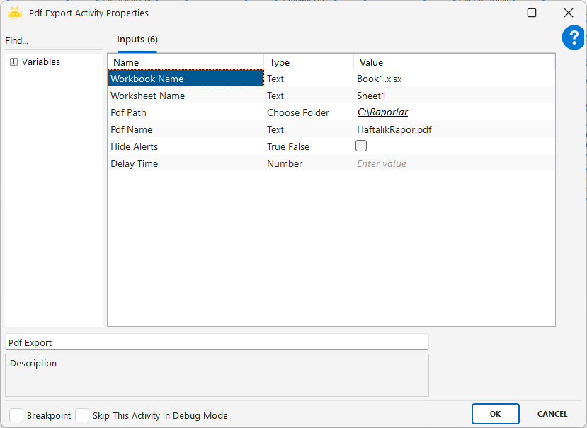
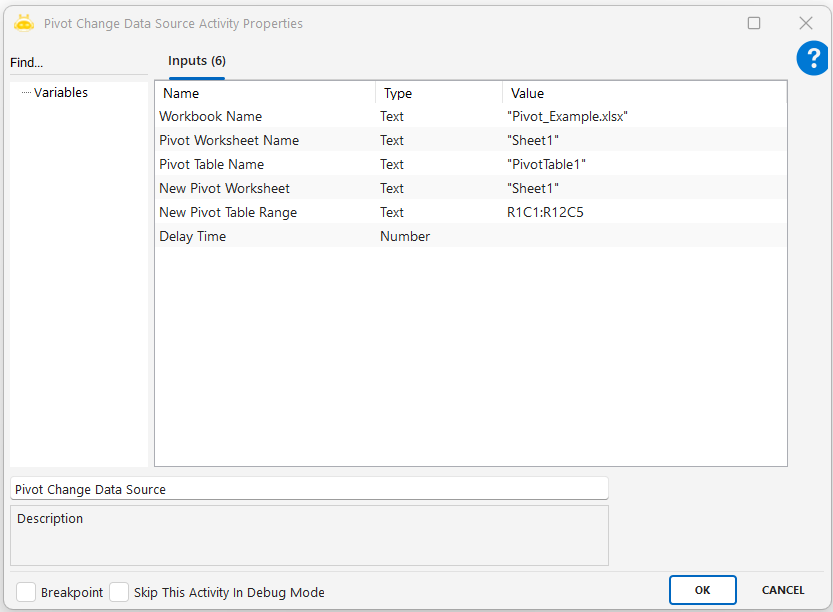
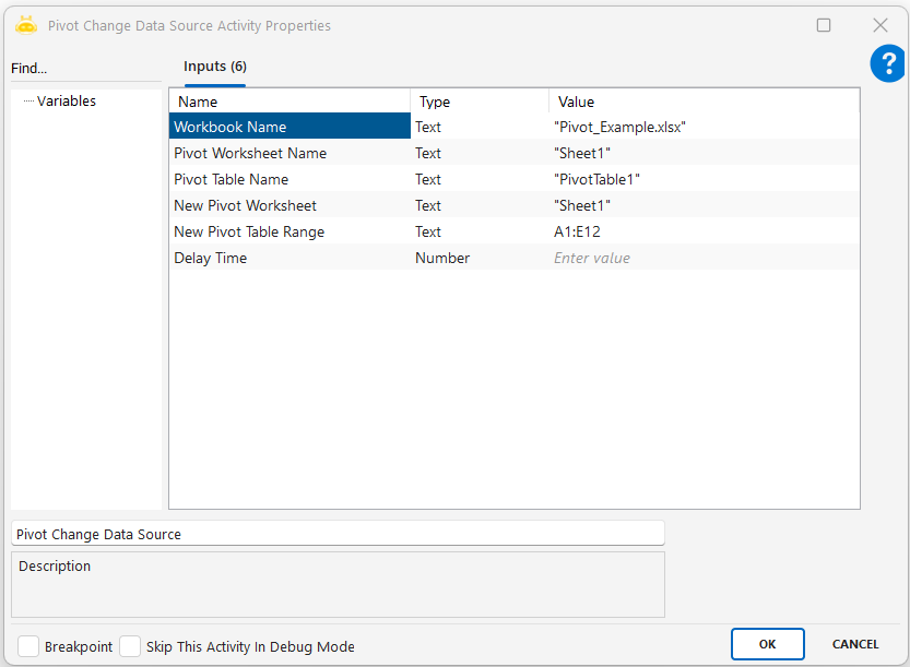
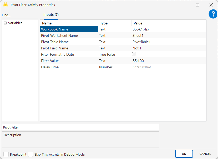
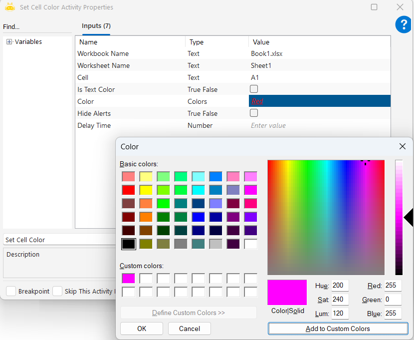
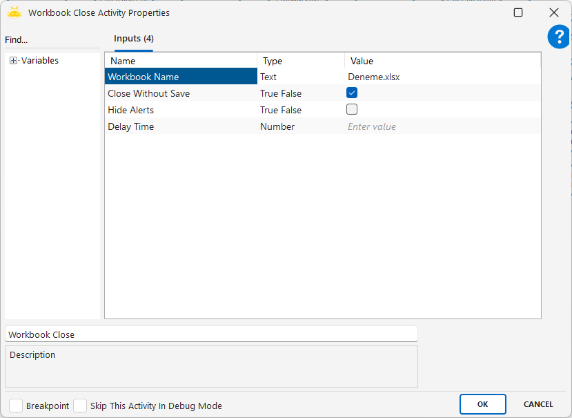
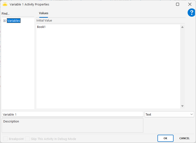
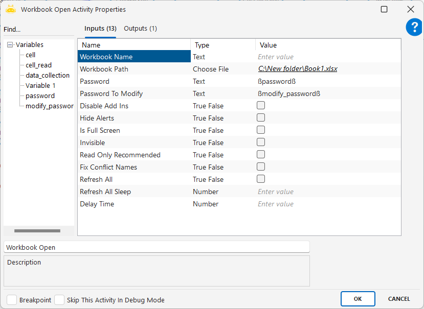
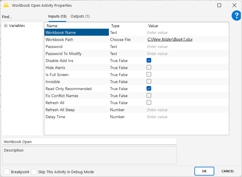
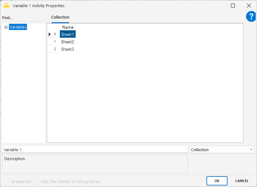
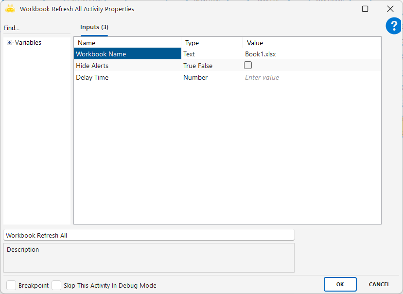
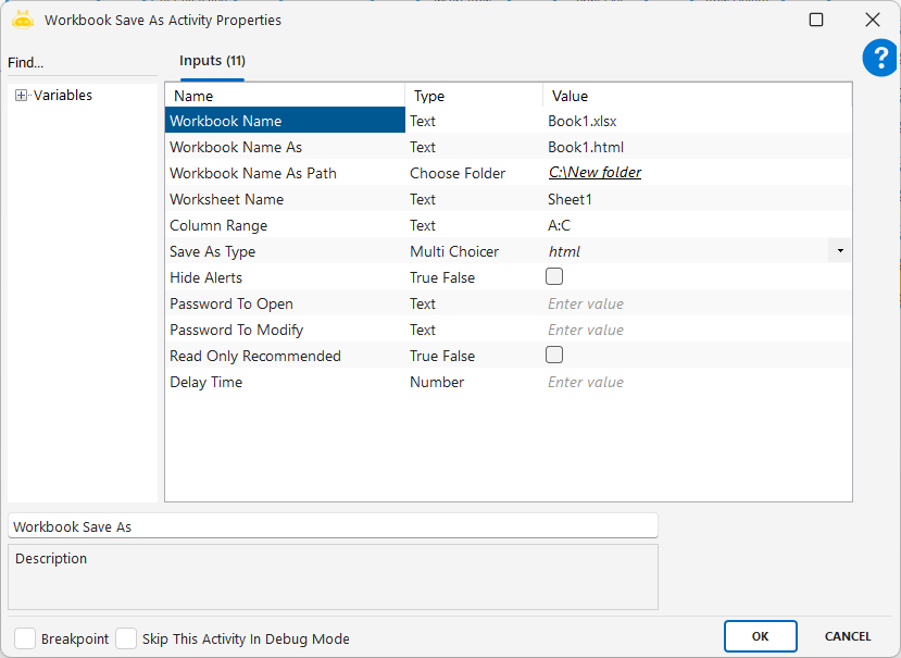
Workbook Name: Name of the Excel file where the new sheet will be created (e.g., Book1.xlsx)
Worksheet Name: Name of the new worksheet to be added (e.g., Rapor2025)
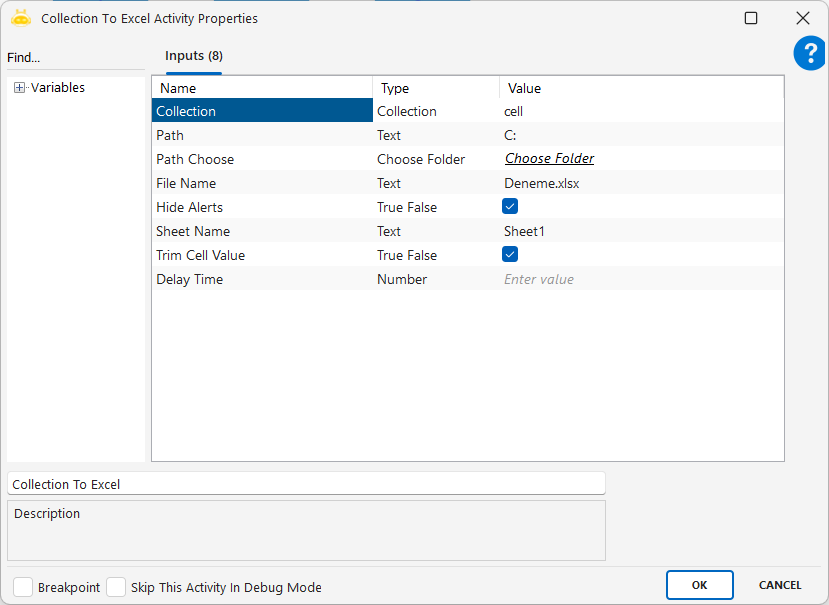
Notes
Workbook Name must include the full file name and .xlsx extension
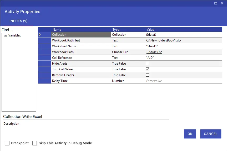
Worksheet Name must be valid:
Maximum 31 characters
Cannot include special characters such as /, *, [, ], ?, etc.
The activity returns an error if a sheet with the same name already exists—use Worksheet Exists beforehand if needed
The operation may fail if the file is open, locked, or in use by another application
The new worksheet is added to the end of the workbook by default